Load profiles is an add-on module to dpPower Analyzer. It allows for the creation of individual and general load profiles based on historical power data from end customers and weather data. Load profiles can be used as input load data in calculations.

 

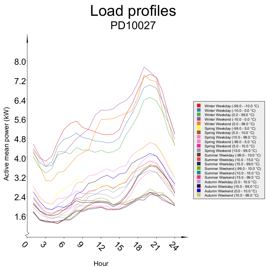
Load profiles are daily curves describing the power usage of an end customer or a secondary/primary substation. The load profiles are divided into groups based on:

•Season

•Day type

•Temperature. Up to four intervals per season.

 

See graph for an example of one customer’s load profiles.

Individual load profiles

Individual load profiles apply to one specific customer and are created based on the historical hourly measurements from the end customer’s meter in combination with weather data. Creation of individual profiles therefore requires Historical measurements to be imported and a weather series of daily mean temperatures - however the add-on module Historical Measurements is not required. See section Historical measurements.

 

Individual load profiles creation guide:

1.Open Analyzer > Administrate load profiles….

2.Select tab Create individual load profiles.

3.Check the box Use selected meters and choose a method of selecting meters:

oSelect from list: Allows the user to search for a specific meter. If the search field is left empty, the search will include all meters in the system.

oSelect in map: Allows the user to place a polygon in the map. When the polygon is completed, right-click and select Define area. All meters inside the polygon will be selected.

oSelect with trace: The trace window opens. All meters included in the trace will be selected.

4.Select Hourly values as Meter type.

5.Activate use date limitations and select a time interval if only values from certain dates should be used in the creation of the load profiles. If it is left unchecked, all saved measurements will be used.

6.Press Start generation.

 

General load profiles

General load profiles apply to a group of end customers and are created from a set of individual profiles.

 

General load profiles creation guide:

1.Open Analyzer > Administrate load profiles….

2.Select tab Create general load profiles.

3.Select which meters should be included as input to the generation, either by:

a.ISIC-code; or

b.Specific meter selection:

•Select from list: Allows the user to search for a specific meter. If the search field is left empty, the search will include all meters in the system.

•Select in map: Allows the user to place a polygon in the map. When the polygon is completed, right-click and select Define area. All meters inside the polygon will be selected.

•Select with trace: The trace window opens. All meters included in the trace will be selected.

    Click OK. The list on the right side of the window is populated with meters.

4.Type a description and an ID for the general profile and press Start generation.

 

Link general load profile to end customer

The codelist MAP_LOAD_PATTERN is used to assign general load profiles to end customers who do not have individual load profiles - for example, in newly developed or planned areas.

Each general load profile in MAP_LOAD_PATTERN is associated with a specific TYPE_CODE, which links it to the corresponding general load profile defined in the LOAD_PATTERN codelist. The TYPE_CODE value must match in both codelists for the mapping to be valid.

Both the MAP_LOAD_PATTERN and LOAD_PATTERN codelists can be accessed via:

Analyzer > Administrate load profiles > tab Administration > Show/update drop-down menu.

A general load profile is selected based on up to four variables: fuse size, energy consumption, ISIC code, and tariff code. Fuse size and energy consumption are specified as ranges.

When multiple variables are defined for an entry in MAP_LOAD_PATTERN, the selection follows this priority:

1.ISIC code

2.Tariff code

3.Energy consumption

4.Fuse size

If an entry in MAP_LOAD_PATTERN includes ISIC code = BASE, it will be used as a fallback. If no matching entry is found, no general load profile will be assigned.

 

How General load profiles are used in calculations

When performing calculations with general load profiles, these profiles are normalized during use, not only during their creation from individual load profiles. This means that the actual calculation results may differ from theoretical values.

The active power, P(t), is calculated using the formula:

P(t) = k(t, season, typical day, temperature) * average hourly energy consumption

•k() - A relative active power factor from the general load profile.

•Average hourly energy consumption - The energy consumption is multiplied by a normalized factor based on the general load profile.

Normalization adjusts general load profiles during calculations to ensure they are based on the average hourly energy consumption and adhere to the parameters defined during their creation.

 

Retrieve all load profiles for a meter

1.Right-click on a delivery point, customer facility or a meter that has load profiles stored.

2.Select Calculated values > Load profile meter graphic. All daily curves that are stored are displayed. Only the active power is presented.

 

Load summed load profiles for a station

Open the right-click menu and select Calculated values > Hourly values > Load profiles, summary. It is possible to filter the load profiles using the filter button in the menu bar.

 

Administration

Individual load profiles can be deleted, either by truncating the entire database table or by only deleting certain selected profiles, from the Administration tab in the Administrate load profiles window.

 

The codelists related to the module are accessed through the Show/update drop down menu in the Administration tab in the Administrate load profiles window.

 

Weather data

For Swedish customers, weather data can be imported using SMHI’s weather API.

 

The integration with SMHI’s API enables automatic retrieval of temperature data from all of SMHI’s weather stations. Using this integration comes with no extra costs for the customer, however since the API is SMHI’s, it is only available in Sweden.

 

Setup:

1.Place the object temperature measurement in the map. All attribute fields can be left empty for now.

2.Open the Query tool > Search > External search services > Weather station (SMHI).

3.Change the max rows and press Search.

4.Find the relevant weather station and copy the Name and Station ID from the Query tool to the “ID” and “Alternative ID” in the attribute form respectively.

 Link to a map of SMHI’s weather stations:

 https://www.smhi.se/vader/observationer/observationer#ws=wpt-a,proxy=wpt-a,tab=vader,param=t

5.Post the changes.

6.Open Analyzer > Administrate load profiles > Reading and run one of the jobs with SMHI in the name.

7.Right click the temperature measurement info object and select Show temperature set. If everything works as intended, the weather series should be presented in a graph.

 

A scheduled job can also be configured by Digpro which imports the previous day’s mean temperature in order to automatically keep the weather data up to date.