1 System earthing / neutral-point equipment in dpPower Analyzer
2 Reactor and resistor data
2.1 Reactor data
If the set current is specified for the reactor, then this value will be used instead of the set current in the code-list (12A and not 15A is selected).
Active losses are calculated according to the active losses in % (of the set current). The result is presented in the report “MV earth fault report” as current contribution from above and from below,Sum resistive current from above A Sum resistive current from below A
(sum of resistive current contribution in direction up and down in the network)
See Appendix: Active reactor losses
2.2 Resistor data
If the set current is specified, this will be used instead of the one that is specified in the code-list. (7A and not 5A is selected).
3. Central compensation
A neutral-point is defined in the primary sub-station, and is equipped with a neutral point reactor and or neutral point resistor.
3.1 Resistance / reactor earthed neutral point in Y or Z vector grouped transformer windings.
Construction / interpretation.
The neutral point is defined with the object Neutral point, which is connected to a winding with the correct vector group.
In the neutral point there is a possibility to add one “additional” capacitive current contribution, a correction term to be used when you know that there is more capacitance current generation in the network than what is received from the calculated network. It is also possible to add one “discrepant” resistance for calculation of high ohm earth fault (Default = 3000 ohm).
Modeling the neutral point system
The neutral point system can be created using a number of objects:
Earthing switches (Earthing disconnectors)
Neutral point Bus bar which is the object that reactors and resistors should be connected to
Earthing Lines (overhead and underground)
Resistors
Reactors
Earthings
This should be enough in order to define most types of earthing systems for a Y or Z-vector grouped transformer.
The data that the earth fault calculation uses is captured from neutral point and reactor / resistor only. The other objects are only used to model different system constructions topologically, such as alternative possibilities for connections with the help of disconnectors and combined neutral point systems for several transformers.
Note! The earthing switches between resistor / reactor and neutral point bus bar can be documented, but it is not necessary to do so.
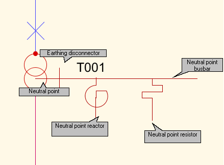
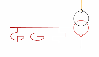
A typical neutral-point configuration for a transformer with a Y or Z vector group.
3.2 Constructed neutral point at a D grouped transformer winding
If the system earthing is a constructed neutral point, i.e. D vector group on 10kV side this can be achieved by adding a “neutral-point former” (neutral-point winding in menus) towards the same 10kV bus bar that the transformer is connected to. Otherwise the neutral-point is constructed as described above.
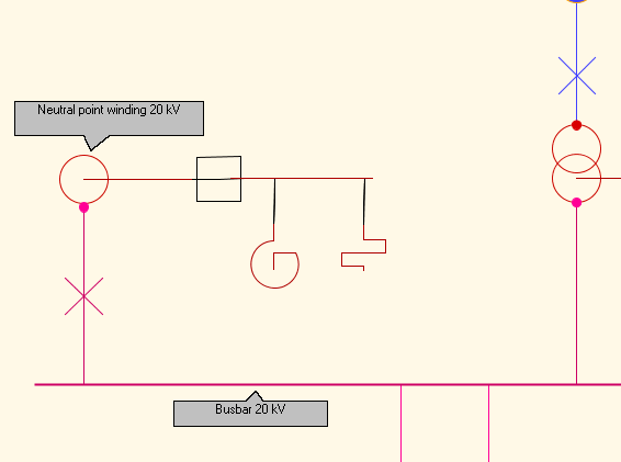
It is not necessary to create a new branch from the bus bar. The neutral point winding can also be added to the same branch as the transformer itself.
4. Local compensation
4.1 Local compensation in secondary substation transformer
There are two methods:
1.The same principle as for the ordinary system neutral-point, complete documentation.
2.Simplified method.
1. Complete documentation with earthing switches between neutral-point and neutral-point bus bar.
If the upper-side of the winding in a substation transformer is Y(N)-connected, then a local compensation can also be achieved by adding a neutral-point against the Y(N)-winding.
2. Simplified method
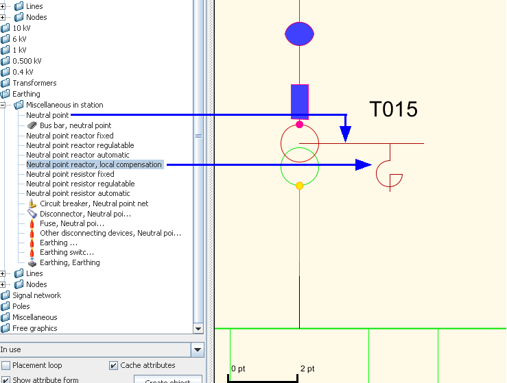
Only create the Neutral-point and Neutral point reactor, local compensation. The local compensation reactor can be connected directly to the neutral-point.
4.2 Local compensation with local neutral point formers
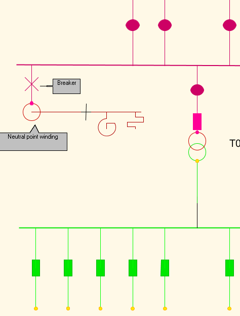
Local compensation connected to a neutral point former (neutral point winding). If the system earthing concerns a local compensation, then this can be achieved by adding a “neutral point winding” connected to a network part, for instance a bus bar. Otherwise the neutral-point is constructed as described above.
5. Parallel reactors
There can be parallel reactors in the neutral-point. Set current will be added for the parallel reactors.
6. Sub-station with several transformers and neutral point systems
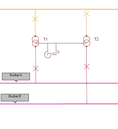
If there are several transformers in the same sub-station they can share the same neutral point system or have two different neutral point systems. The result for each neutral point can be presented per transformer in the HV Earth-fault report.
7. Moreover
If neutral point equipment is missing, then it is assumed that the MV network has an isolated earthed neutral point and that the LV network is directly earthed.
Reactor Losses
Active reactor losses
Serial presentation
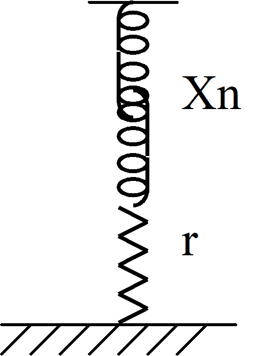
The active losses of a reactor (winding) can be represented as a small resistance r in a series with the reactance Xn where…
(1)
r = p Xn
p = tan б (= r / Xn) = the loss-factor of the reactor (= r I²m / (Xn I²m)
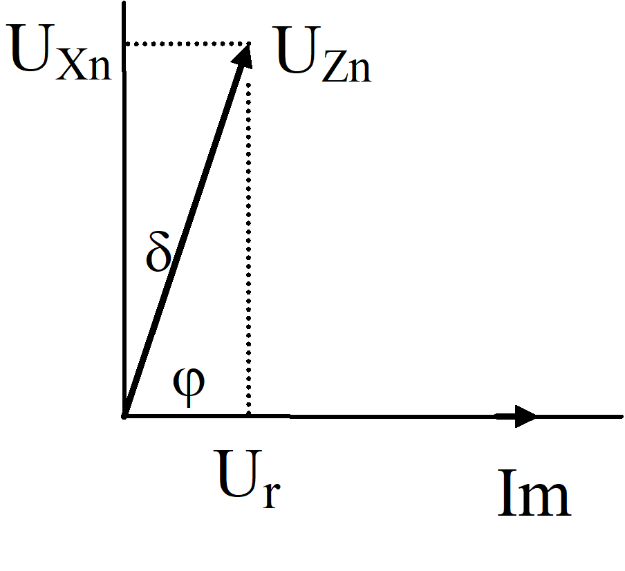
б = 90° - φ = the loss-angle of the reactor
¦Zn¦= Xn (1 + (r / Xn)²)½= Xn (1 + p² )½ = Um / √3 / Im
Um is the rated current of the reactor (main voltage) ; ¦UZn¦= Um / 3
Im is the rated current of the reactor.
Which gives…
Zn = r + jXn
Yn = 1 / (r + jXn) = (p Xn - jXn) / (p² X²n + X²n)
= (p - j) / ( p²+ 1) / Xn
R’ and X’ should be equivalent
![]()
Yn = 1 / R’ - j 1 / X’ (2)
Identification results in...
1 / R’ = p / (p²+ 1) / Xn ; R’ = (p² + 1) / p Xn (Xn/p = X²n / r If p << 1)
1 / X’ = 1 / (p² + 1) / Xn ; X’ = (p² + 1) Xn (Xn)
Stored as neutral-point data RSH( ) = R’ ; XSH( ) = X’
Parallel representation
The losses can also directly be represented as a large resistance R parallel to the reactance X
Loss factor p = R IR² / (X IX² ) (3)
= X / R
where…
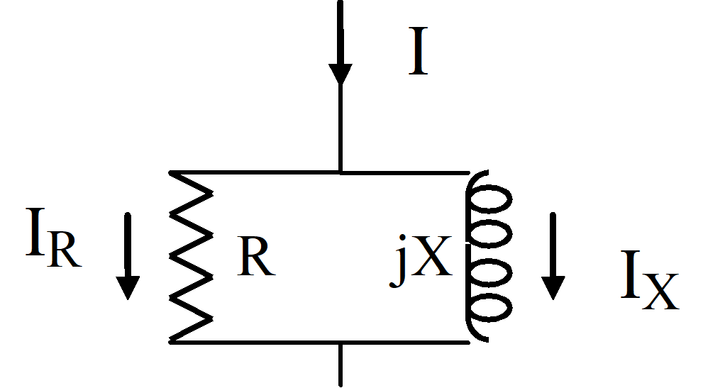
IR = jX / (R + jX) I ; IX = R / (R + jX) I
IR² = IR I* R ; IX² = IX I*X ; IR² / IX² = X² / R² = p², i.e. p =│IR│/│IX│
From (1) and (3) the following is obtained… (4)
p = r / Xn = X / R = ¦IR¦ / ¦IX¦) if p<<1 then Xn = X
R│IR│ = X│IX│ = Um / 3
Re-calculating parallel- to serial circuit results in (re-calculating of serial- to parallel is at (2))
Z = r + jX RjX / (R + jX) = (RX² + j R²X) / (R² (1 + X² / R²)) (5)
= X² / R + jX if p << 1
For the parallel circuit can X be obtained from rated data according to…
│IX │X = │R / (R + jX)│Im X = 1 / (1 + p²)½ Im X = Um / √3
X / (1 + p²)½ = Um / √3 / Im
To summon up, this shows the correlation (1) – (5) that, if p << 1 then there is a serial representation r of the losses, equivalent to the parallel representation R = X² / r, and a parallel representation R is equivalent with a serial representation r = X² / R.
Independent of the size of p, the active losses can freely be represented via serial- or parallel representation. For large values of p, the reactances Xn and X will be different, but X’ and X will be different even then, and so also R’ and R.
X’ = (1 + p²) Xn
= (1 + p²) / (1 + p² )½ Um / √3 /Im
= (1 + p² )½ Um / √3 / Im
= X
Reactive power at serial QS- and parallel QP – representation
QS = Xn I²m
= Um / √3 / (1 + p² )½ Im
QP = X I² X
= X R² / (R² + X²) I²m = X I²m / (1 + p² )
= Um / √3 / (1 + p² )½ Im