Fault mode determination

 

Fault-mode determination of single-phase to ground fault is done iterative in two steps, where each step is repeated until the fault impedance and the fault mode is determined.

 

1.Calculation of the earth fault impedance Zj with the help of a model with approximate network representation (as described in section 1).

2.Calculation of earth fault currents with the help of a complete network representation (as described in section 2, with Zj from the step 1 above).

 

 

1.Model with an approximate network representation

 

Approximate series impedance Z’ for a single phase earth fault

 

Z’k = 2 Z’+k + Z’0k        (1.1)

 

where…

 

Z’+k = resulting positive sequence impedance in node point k

 

Z’0k = Z0t + Z+Lk + 3 ZNk

 

= approximately, resulting zero sequence series impedance in node-point k

 

Z0t = the transformer zero sequence impedance

 

Z+Lk = positive sequence serial impedance from the transformer neutral point to the node point k

 

ZNk = neutral conductor / shield  impedance from the transformer neutral point to the node point k

 

Single phase earth fault currents IR written as

 

(1.2)

IR = 3VR0k / (Z’k + 3 (Z’n + Zjk))

(1.3)

   = VR0k / (Z’k / 3 + Z’n + Zjk)

 

where…

 

VR0k is the voltage in phase R in the fault location k before the earth fault occurs.

Zjk is the earth fault impedance in the fault location k.

Z’n is the neutral  point impedance Zn in parallel with the capacitive neutral earth reactance (1 / (3jwC0)

 

For representation of the approximate series impedance in the equivalent below, the notification ZEJ is used for the series impedance including the earth fault impedance, ie

(1.4)

ZEJ = Z’k / 3 + Zjk

 

1.2 Calculation of earth-fault-currents with the approximate model

 

 

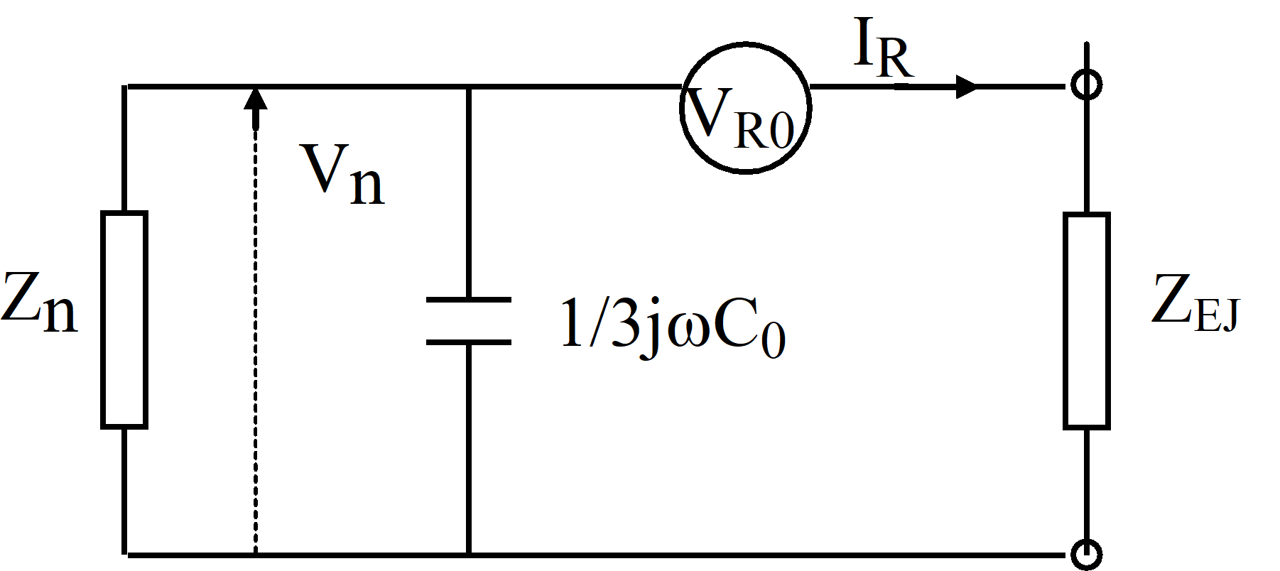
Figure 1.1. Approximate equivalent for single phase earth fault

 

From the equivalent the following is obtained

(1.5)

IR = VR0 / (ZEJ + Z’n)

 

where…

(1.6)

1 / Z’n = 1 / Rn + j(3wC0 – 1 / wLn)

 

Rn also includes, besides neutral point resistors, resistance’s that represents the resistive losses of the neutral point reactors, including also those located outside the primary substations.

 

Ln also includes inductances for neutral point reactors located outside the primary substations

 

C0 also includes other measured capacitive current, including also neutral points located outside the primary , recalculated at nominal voltage.

 

Neutral  point (zero sequence) voltage will be

(1.7)

Vn = - IR * Z’n = - VR0 / (ZEJ / Z’n + 1)

 

    = k * VR0

 

where…

(1.8)

k = 1 / (ZEJ / Z’n + 1)

 

At negligible earth fault impedance ZEJ the factor k = 1.

 

The earth fault current divided on radials is illustrated by Fig. 1.2.

 

 

 

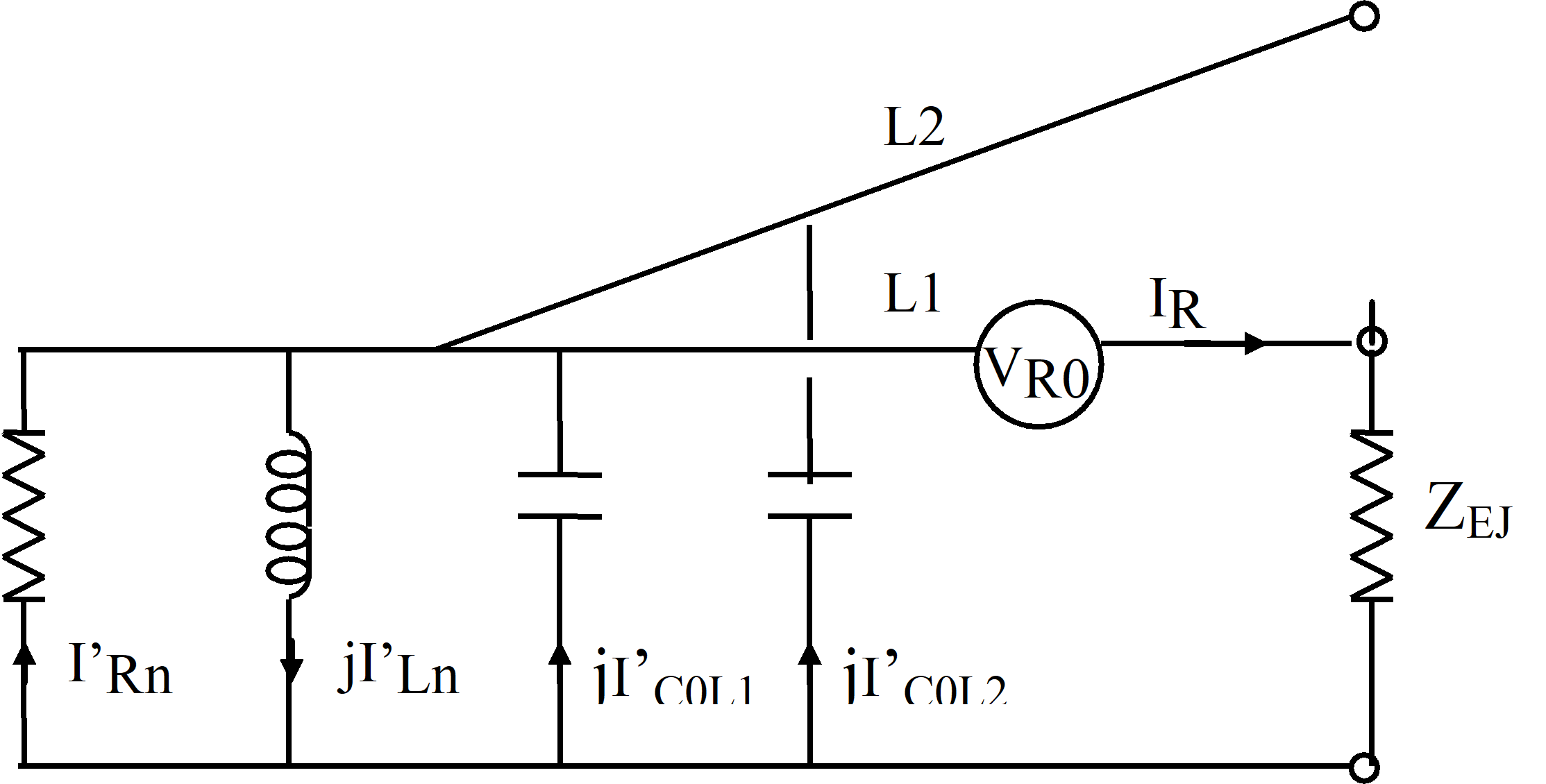
Fig. 1.2  The division of the earth-closing current in radials

 

At a fault on radial L1 the current passes through the conductor protection

(1.9)

L1)        I’L1 = k IL1 = k (IRn- IRnL1 + j(IC0 - IC0L1 - ILn + ILnL1))

(1.10)

L2)        I’L2 = k IL2 = -k (IRnL2 + j(IC0L2 - ILnL2))

 

Where the current contribution also comes from the neutral zero-points located outside the primary substations, including active reactor losses and other measured capacitive current

 

 

 

2.Complete model with network capacitances and neutral points located outside the primary substations, with Y-matrix representation of the network

 

Network representation with factored Y-matrixes (positive- and zero sequence).

 

In an electrical power network the correlation between currents and voltage is written as

 

YV = I                (2.1)

 

where

 

I = vector of node point currents

V = vector of node point voltages

Y = G + jB = node point admittances matrix of the network

G = conductance ; B = susceptance

 

 

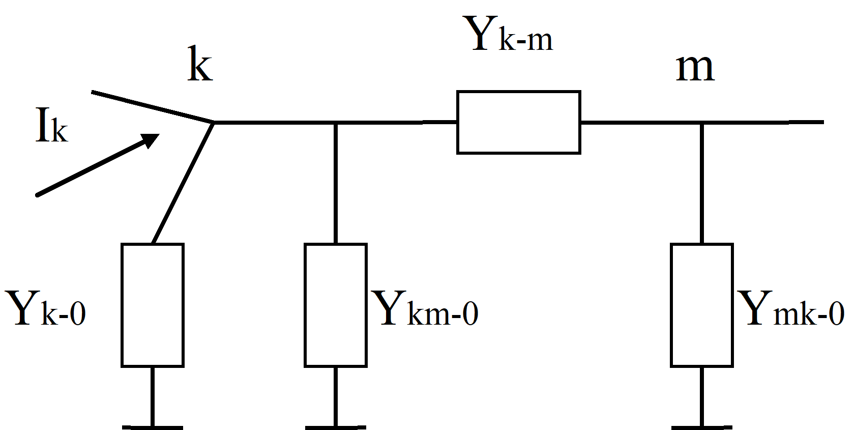
 Fig. 2.1.  Representation of an electrical network

 

The network elements are represented as π links according to figure 2.1, where…

 

Yk-m = π equivalent series admittance for section k-m

Ykm-0 = π equivalent shunt admittance i node-point k for section k-m

Ykm-0 = ditto for node-point m

Yk-0 = admittance for shunt element in node-point k (capacitor, reactor, generator)

 

Injected node point current Ik is written as

(2.2)

Ik = Vk Yk-0 + Vk SmYkm-0 + Sm(Vk - Vm)Yk-m

  = (Yk-0 + Sm (Ykm-0 +Yk-m))Vk - Sm Yk-m Vm

 

Where the summation is done over all node-points m that are directly connected to node-point k.

 

The admittance matrix diagonal element and the non-diagonal element i  (2.1) is according to (2.2)

(2.3)

Ykk = Yk-0 + Sm (Ykm-0 +Yk-m))

Ykm = - Yk-m

 

Correlation (2.1) can also be written as

(2.4)

V = Y-1 I

  = Z I

 

where

 

Z = R + jX = the node-point impedance matrix of the network

R = resistance; X = reactance

 

When simulating errors in a given point of the network, the actual column of the Z-matrix is calculated out from the Y-matrix. This is written as…

(2.5)

Z(k) = Y-1 E(k)

 

where E(k) is the column k in the unit matrix with a digit one in position k and zero digits in the other places. It can also be interpreted that an injection of a p.u. current in a node-point k gives node-point voltages that are identical with the corresponding column in the Z-matrix.

 

When calculating (2.5), a matrix factoring is applied, which in this case will be a LDU factoring of the linear equation system (2.1) which can be written as

(2.6)

A x = b

 

Factoring of A gives

(2.7)

LDU x = b

(2.8)

U x = y

(2.9)

LD y = b

 

where…

 

- L and U are upper and lower triangular matrixes with the digit one in the diagonals

 

- D is a diagonal matrix

 

- help-vector y is solved for the right side b with a ’fast forward’ (FF) substitution and division with D, according to the correlation (2.9)

 

- vector x is solved with a ’backward’ (B) or, a subset of the x-elements are desired, with a ’fast backward’ (FB) substitution

 

The method described above for the Y-matrix is used when calculating a single phase earth fault, when one want to represent the network as π links, where the conductor capacitors and the network localized neutral points are represented as shunts in the node points (see Fig. 2.1).

 

When calculating earth faults in a node-point k the positive sequence and zero sequence  - Z-matrix-columns Z+(k) and Z0(k) for the node-point (positive- and negative sequence  impedances assumed to be equal) after which the currents in the fault location is calculated as                (2.10)

I+k = I-k = I0k = V+k0 / (2 Z+kk + Z0kk+ 3 Zjk)

 

The voltage in a node-point m in the network is calculated as                

V+m = V+m0 - Z+km I+k        (2.11)

V-m = - Z+km I-k                (2.12)

V0m = - Z0km I0k                (2.13)

 

The impedances Z+kk, Z+km och Z0 kk, Z0km are elements in each of the columns Z+(k) and Z0(k)

 

 

Fault in a conductor section

 

When you want to calculate fault-currents for faults out on a conductor section between two node-points, for instance as in the example below – a fault-mode determination method like below is used

 

 

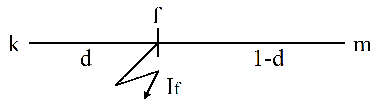
Fig. 2.2 above illustrates a fault in a point f out on the conductor section k-m, on the distance d from node-point k. The following correlation between currents and voltages can be determined

(2.14)

Vf = Vk - d Zk-m Ik-f

(2.15)

Vf = Vm - (1-d) Zk-m Im-f

(2.16)

If = Ik-f + Im-f

 

The correlation between (2.14) and (2.16) gives…

(2.17)

Vf = Vk - d Zk-m If  + d Zk-m Im-f

 

The solution of Im-f  from (2.15) and insertion in (2.17) gives…

(2.18)

Vf = Vk - d Zk-m If  + d Zk-m ((Vm - Vf) / ((1-d) Zk-m))

   = (1 - d)Vk + dVm - d(1 - d) Zk-m If

 

If 1 p.u. current is injected into point ‘i’ the current in 'f' will be…

(2.19)

Vif = Zfi = Vik - d Zk-m Iik-m

 

    = Vik - d(Vik - Vim)

 

    = (1-d)Zki + d Zmi i = 1, 2, ….. , n

 

where the upper index ‘i’ indicates that the quantity derived from the 1 p.u. injection in node-point ‘i’ and n indicates the number of node points in the network.

 

If 1 p.u. is injected in point f the following correlation according to (2.18) will be obtained…

(2.20)

Vff = Zff =(1-d) Vfk + d Vfm + d(1-d) Zk-m

 

= (1-d) Zkf + d Zmf + d(1-d) Zk-m

 

Insertion of (2.19) in (2.20) with i=k and i=m gives…

(2.21)

Zff = (1 - d) / ((1 - d) Zkk + d Zmk + d((1 - d) Zkm + d Zmm) + d(1 - d) Zk-m

   = (1 - d)2 Zkk + 2d(1 - d) Zkm + d2 Zmm + d(1 - d) Zk-m

 

The expressions (2.19) and (2.21) shows how the impedance matrix column for the fault location f out on the conductor section k-m is obtained with the help of the impedance matrix columns for the end points and the sections own impedance.

 

For a simple radial network without shunt elements, for instance the approximate network in section 1, is Zkm = Zkk and Zmm = Zkk + Zk-m. Insertion of these values in (2.21) gives

(2.22)

Zff = Zkk + d Zk-m

 

 

3.Algorithm for fault-mode determination

 

3.1 Estimation of earth fault impedance

 

The value of the parameter k is calculated from the earlier three correlations (1.7), (1.9) and (1.10)…

(3.1)

k = - Vn / VR0

(3.2)

k = I’L1 / IL1

(3.3)

k = I’L2 / IL2

 

where (3.1) relates to the neutral point, (3.2) relates to the faulty radial, and (3.3) relates to the healthy radials.

 

Vn , I’L1 and I’L2 are measured values with unknown fault impedance and unknown fault-mode.

 

- VR0 , IL1 and IL2 are calculated values from the approximate model (equivalent) with the fault-impedance ZEJ = 0.

 

According to the correlation (1.8), k = 1/ (ZEJ / Z’n + 1) which gives

(3.4)

ZEJ = Z’n (1-k) / k    

 

ZEJ is calculated from each of the correlations (3.1), (3.2) and (3.3), and a mean value is created.

 

After that, Z’k is calculated from the approximate network representation, according to the correlation in (1.1), after which the fault impedance is created from the expression (1.4) as

(3.5)

Zjk = ZEJ - Z’k / 3

 

and 3 Zjk is inserted in the complete model in the expression (2.10) for single phase earth fault.

 

In the first iteration, before any possible fault mode has been determined, the Z’k is calculated as a mean value over the node points in the network. In the following iterations, the fault-mode comes from the complete model, ie, the actual section k-m and position d, and is inserted into the expression (2.22) for the radial network.

 

 

3.2 Calculation of fault mode

 

Calculation of fault-mode is done with the complete model 2 and starts with determination of border sections k-m in the faulty radial. A border section is defined as a section k-m, such as

 

- A fault in node-point k gives a fault current I0fk that result in a fault current out on the radial, which is equal to or greater than the measured current I’r

 

- A fault  in node point m gives a fault current I0fm that result in a fault-current I0rk out on the radial which is less than measured current I’r

 

The current I0fk and I0fm is calculated from the correlation (2.10), and the currents I0rk and I0rm are calculated from the neutral sequence voltages, and according to the correlation (2.13) for the node point rk and rm (m=rk and  m=rm) inserted into (2.13))  , and the neutral sequence π link of the section.

 

When determining the fault-mode f on a section, the calculation is performed according to the principles as described in section 2.2, where the correlations (2.19) and (2.21) are used for calculating positive- and neutral sequences of the impedance-matrix-columns for the fault-point f. The positive- and neutral sequence impedance  Z+ff and Z0ff are used for calculating the fault-current I0f. The neutral sequence impedances Z0f rk and Z0f rm are used for calculating the neutral sequence voltages of the node points rk and rm in the measured sections. And with these voltages and the neutral sequence π link of the section, the fault-current I0rf is calculated on the radial.

 

The distance d to the fault point f is determined by an interval division.

 

A1) Assume dmin = 0 and dmax = 1

A2) d = 0.5 (dmin + dmax ), if (dmax - dmin) ) < eps1 then the fault-mode has been identified

 

A3) calculate the fault-current I0rf out on the radial at the fault mode d

 

A4) if I0rf is equal to measured current I’r, or (I’r -I0rf) < eps2 ), then the fault mode has been identified

 

A5) if I0rf is greater than measured current I’r, then dmin = d is inserted, select A2

 

A6) if I0rf is less than measured current I’r, then dmax = d is inserted, select A2

 

When calculating the fault-mode according to section 3.2, the absolute value of the currents are used.

 

When the fault mode has been identified, then the earth fault impedance is corrected Zjk = ZEJ - Z’k / 3 above, (the correlation (3.5)) with an approximate series impedance Z’k / 3 that is recalculated via insertion of the fault-mode into the calculation of the impedance (2.22) for radial network.

After that a new iteration starts with the fault mode determination. When the changes of the earth fault impedance, from one iteration to another, is less than a given limit value, the iterations stops and the fault-mode for this border section is considered to have been determined.

 

If the faulty radial has several border sections (possible fault locations) the iterative process (3.2) starts again.